RGEES Nonresponse Bias Analysis Supporting Analyses
RGEES NRBA Supporting Analysis.docx
Recent Graduates Employment and Earnings Survey (RGEES) Standards and Survey Form
RGEES Nonresponse Bias Analysis Supporting Analyses
OMB: 1845-0138
Page
Postsecondary programs subject to the gainful employment regulations may appeal program-level debt to earnings (D/E) ratios calculated by the Department (34 CFR Parts 600 and 668). The earnings component of the D/E ratio is provided by the Social Security Administration, but institutions may calculate an alternative earnings measure by obtaining state employment records or by administering an earnings survey to program graduates. Institutions that choose to submit alternate earnings appeal information based on survey data will survey all Title IV funded students from programs who graduated during the same period that the Department used to calculate the D/E ratios, or a comparable period as defined in 668.406(b)(3) of the regulations. The survey will provide an additional source of earnings data for the Department to consider before determining final D/E ratios for programs subject to the gainful employment regulations. Programs with final D/E ratios that fail to meet the minimum threshold may face sanctions, including the possible loss of Title IV federal student financial aid program funds.
The National Center for Education Statistics (NCES) of the U.S. Department of Education (Department) is required by regulation to develop an earnings survey to support gainful employment (GE) program evaluations (see 34 CFR 668.406 as specified in final regulations published in the Federal Register in October 2014). The regulations specify that the Secretary of Education will publish in the Federal Register the survey and the standards required for its administration. Thus, NCES developed the Recent Graduates Employment and Earnings Survey (RGEES) and related Standards for use in a debt-to-earnings (D/E) appeal under the GE regulations as an alternative to the Social Security administration earnings data.
The RGEES standards specify that the response rate for an individual program must be at least 50 percent for the data to be used to support an appeal under the Gainful Employment Regulations appeal process;1 and that a nonresponse bias analysis must be conducted if the unit response rate is between 80 percent and 50 percent.2
Two questions motivated the research that follows:
Are there any available data that are sufficiently correlated with student earnings as to be useful in evaluating the impact of nonresponse on respondent earnings?
What level of relative bias in the identified variables is acceptable?
As a first step, NCES investigated the extent to which available variables are correlated with the variable of interest in this survey – earnings of program graduates. The results from this first step were then used to develop a proposal for variables around which to construct nonresponse bias analyses.
Data
Program participants who receive Title IV funding filed a Free Application for Federal Student Aid (FAFSA) and these data are retained in ED’s National Student Loan Data System (NSLDS). Data from NSLDS were provided to NCES by the Department’s Office of Planning, Evaluation, and Policy Development (OPEPD). These datasets were the same ones used for the analysis in support of the GE Regulations.3 The information was aggregated to the program level before data were shared with NCES. Earnings information was similarly aggregated and was provided through OPEPD from the Social Security Administration. The following variables were included in the analyses. Variable names are in parentheses.
2011 Calendar Year Earnings from SSA (Earnings)
Percentage of graduates that received Pell Grants (Percentage Pell)
Percentage of graduates who had an Expected Family Contribution of zero in the academic year prior to graduation (Percentage zero EFC)
Percentage of graduates who were married while in school (Percentage married)
Percentage of graduates who were independent students in the academic year prior to graduation (Percentage independent)
Percentage of graduates who were veterans (Percentage veterans)
Percentage of graduates who were over 24 years of age at graduation (Percentage over 24)
Percentage of graduates who were female (Percentage female)
Percentage of graduates with a mother that had earned at least a bachelor’s degree (Percentage with mom with a BA)
Percentage of graduates with a father that had earned at least a bachelor’s degree (Percentage with dad with a BA)
Analysis of Potential Variables for Inclusion in the Nonresponse Bias Analysis4
To assess the potential for each variable to be used in a bias analysis, NCES examined Pearson r zero order correlations and descriptive regressions. As shown in Table 1, most measures selected for this analysis are correlated to some extent with earnings, the variable of interest. Pearson r correlations range from .015 to 0.611 with percentage of graduates with Pell grants, percentage with ZEFC, percentage veterans, and percentage with a father with at least a BA having correlation values over 0.4 (absolute correlations are referred to here for ease of interpretation).
To better understand the shared contributions of these variables to the variability of income, and to control for possible colinearity between these factors, NCES specified several linear regression models. The first model included the full set of NSLDS-based student characteristics. As shown in Table 2, most variables were statistically correlated with income after controlling for other available variables. Controlling for other variables, the percentage of graduates with Pell grants, who had ZEFC, and who were married had absolute Beta coefficients above 0.2, while the percentage who were over age 24, the percentage who were independent, and veterans had absolute Beta coefficients between .15 and .2. The results also suggested that there is a significant problem with multicolinearity between the percentage of graduates who were independent and the percentage that were over 24. The two variables have variance inflation factors near or above 10, which can indicate such a problem. This is not surprising, since being over 24 is one of the main criteria for being an independent student.
Table 3 shows the average percentage of graduates for each program by graduate characteristic. On average, programs had just over three percent of graduates who were identified as veterans. As a result, even for programs with relatively large graduating classes, a small difference between the estimate for Veterans compared to the actual value for Veterans could result in very large biases that would not be representative of much of the graduating class.5 Thus, because relatively few recent graduates are identified as Veterans, the percent of graduates who were veterans was removed.
Table 4 shows the regression model without the percentage Veterans variable. The overall adjusted model R2 dropped from .517 to .502, indicating a loss of approximately 3 percent of variance explained by the exclusion of the Veterans variable. To identify variables significantly contributing to the remaining R2, product measures were evaluated for each of the remaining variables. Table 5 shows those results. Product measures are the product of each variable’s zero order correlation with the dependent variable of interest (see the 2011 earning column in table 1) and the Beta coefficient from the regression model (table 4). Results from the analysis show that the two variables that were generating concerns about multicolinearity—the percentage of graduates who were independent and of graduates who were over 24—contribute limited information to the overall model. Combined, they account for 6 percent of the R2 of the overall model.6 Table 4 also showed that the percentage of graduates whose mothers had bachelors’ degrees was not a significant predictor.
The remaining variables contributing to more than 5 percent of the model R2 were the percentage of graduates who had Pell Grants, who had zero EFC, who were married, who were female, and who had dads who had a bachelor’s degree. Table 6 shows these 5 variables regressed on earnings. The 5 variables are each significant. The model R2 and adjusted R2 are .497 for a slight reduction of about one-half of a percent in R2 from the larger model with Veterans dropped, indicating a loss of approximately 4 percent of variance explained by the exclusion of the percentage of graduates who were independent, the percentage of graduates who were over 24, and the percentage of graduates whose mothers had bachelors’ degrees.
One further consideration is flexibility in the regulations about the appeals process that will allow programs to add graduates to cohorts that were not in the original cohort vetted with ED. For programs to do this, they will need to independently draw demographic information about cohort members necessary for the bias analysis from either their institutional records or from FAFSA. There is also an open question as to whether the appealing program will be required to independently draw demographic information about cohort members necessary for the bias analysis from either their institutional records or from FAFSA. As a result, limiting the number of variables needed for the bias analysis reduces the potential burden on the appealing programs. The variables about marital status and about fathers with a bachelor’s degree each represent, on average, 30 percent or less of the average graduating class (table 4). Because the events measured by these variables occurred less often and would thus contribute disproportionately more to relative bias, they were selected for removal. The final set of variables recommended for bias analyses are then the percentage of graduates who had Pell Grants, who had zero EFC, and who were female. These three variables, when regressed on earnings, generate an adjusted model R2 of .406 (table 7). This represents a 21 percent reduction in variance accounted for compared to the model with all 10 available variables, and an 18 percent reduction in the variance explained in the reduced form best fit model. While there is a significant reduction in the adjusted R2, the remaining variables represent a reduced data burden on appealing programs, and avoid problems with the inclusion of variables that are relatively less common across program graduates.
Response Rates and Nonresponse Bias Analysis
The Recent Graduates Employment and Earnings Survey (RGEES) includes data on different types and sources of earnings (see RGEES in Attachment A). Given the intended use of the RGEES data, for a case to be defined as a respondent, one or more components of the earnings questions must be answered.
The unit response rate (TR) for RGEES is the number of graduates in the cohort who responded (NR) divided by the total number of graduates in the cohort (NT).
TR = (NR/ NT) Equation 1
Similarly, the unit nonresponse rate (TNR) for RGEES is the number of graduates in the cohort who did not respond (NNR) divided by the total number of graduates in the cohort (NT).
TNR = (NNR/ NT) Equation 2
Note that the nonresponse rate can also be expressed as the inverse of the response rate.
TNR = 1 - TR Equation 3
To understand the elements included in a nonresponse bias analysis, it is important to define several additional measures. The difference between the respondent (YR ) and nonrespondent (YNR) means is as follows.
DNR = YR - YNR Equation 4
Bias due to nonresponse (BNR) is the product of the nonresponse rate (TNR) and the difference
_ _
(DNR) between the mean of the respondents (YR) and the mean of the nonrespondents (YNR) for
_
the variable of interest (Y).
_ _
BNR = TNR (YR - YNR) = TNR (DNR) Equation 5
The relative bias due to nonresponse (RBNR) is the bias (BNR) divided by the mean of the variable
_
of interest for the total population (YT).
_
RBNR = BNR/ YT Equation 6
The relative difference of the means is then the difference (DNR) divided by the mean for the total
_
population (YT).
_ _ _ _
RDNR = (YR - YNR)/ YT = DNR/ YT Equation 7
For RGEES, the total population means for the three variables identified in the exploratory regression analysis were used in an analysis of nonresponse bias. A series of “what if” analyses were conducted for each of the three variables—the percentage of graduates who had Pell Grants, who had zero EFC, and who were female, to evaluate the effect of nonresponse on bias at specific levels of response and with assumptions of varying sizes of the difference between the means for respondents and nonrespondents.
“What if” analysis 1
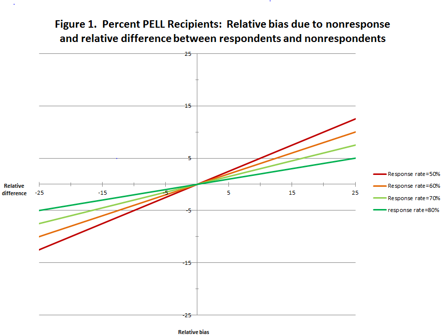
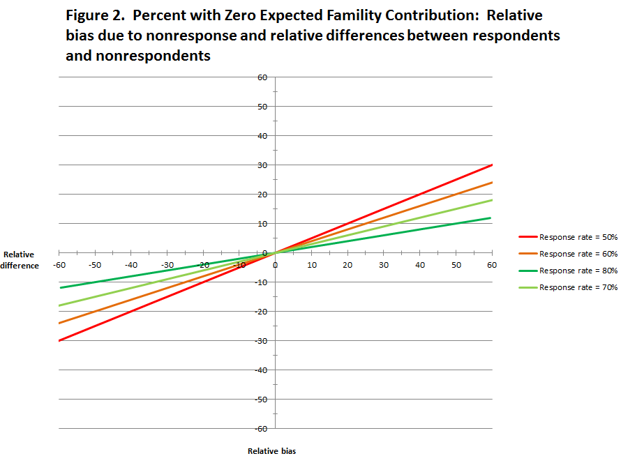
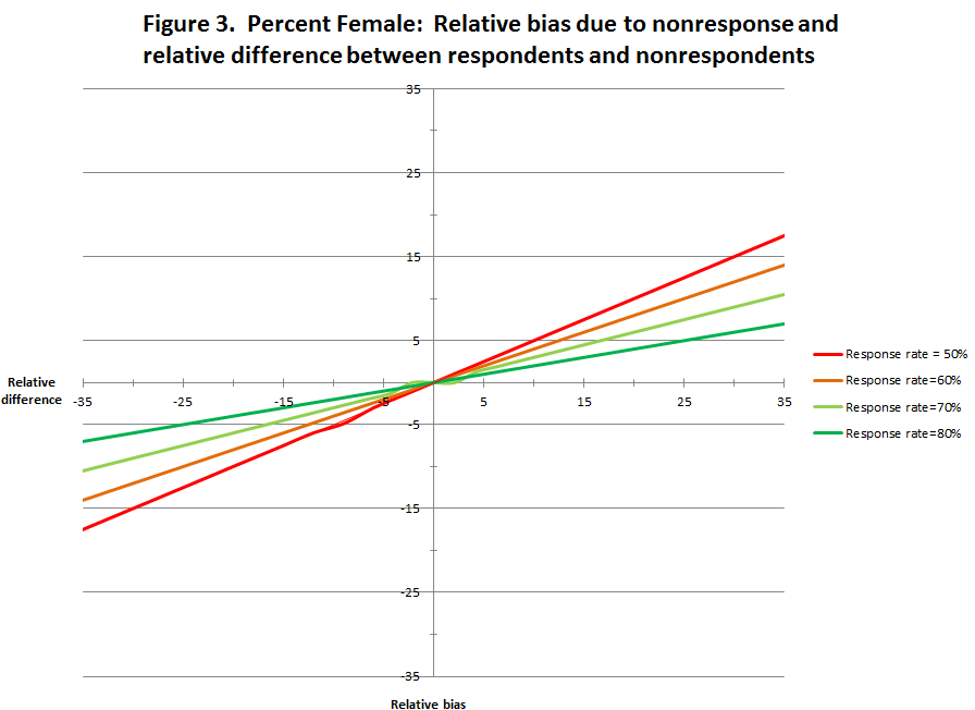
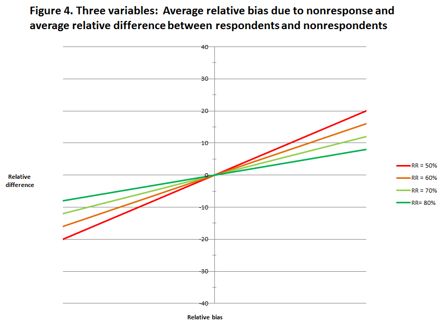
Estimates of relative bias and the relative distance between respondents and nonrespondents were examined to understand how nonresponse error contributes to survey bias under these different assumptions. This was done by first identifying a program at or near the mean for each of the three variables and then using the data for those programs in set of “what if” analyses that produce estimates of relative bias and relative distance at specific response rates (50, 60, 70, and 80 percent),7 with assumptions of varying sizes of the difference from the mean of increasing and decreasing percentage points (1, 2, 3, 4, 5, 6, 7, 8, 9, 10, 15, 20). The results of the “what if” analyses are displayed in Figures 1-4; in each figure the relative bias is plotted on the y-axis and the relative difference between respondents and nonrespondents is plotted on the x-axis. There are separate lines in each figure for response rates of 50, 60, 70, and 80 percent. Figure 1 displays the data for the percent of graduates with Pell Grants, figure 2 displays data for the percent of graduates with zero expected family contribution, figure 3 displays data for the percent of graduates who are female, and figure 4 displays data averaged across the three variables.
By way of comparison, the data in figure 2 show that for graduates with zero expected family contribution with a response rate of 70 percent, a relative difference of 20 percent is associated with a relative bias of 6 percent; however if the response rate drops to 50, a relative difference of 20 percent is associated with a relative bias of 10 percent. In this example, with a 70 percent response rate, the relative difference of 20 percent points and relative bias of 6 percent is associated with a difference of 6 points between respondents and nonrespondents. While, with a response rate of 50 percent the relative difference of 20 percent points and relative bias of 10 percent is associated with a difference of 4 points between respondents and nonrespondents. Thus, while these figures demonstrate that bias due to nonresponse is not just a function of nonresponse; the figures also show that for a set value of the relative difference, the relative bias increases as the response rate decreases.
Looking at this another way using the average across the three variables (figure 4), Taking an actual difference of 5 percentage points if the response rate is 80 percent, the relative difference is approximately 10.8 percent and the relative bias is about 2.2 percent, with a response rate of 70 percent the relative difference increases to 12.4 percent and the relative bias increases to 3.7 percent, with a 60 percent response rate an actual difference of 5 points is associated with a relative difference of 14.5 percent and a relative bias of 5.8 percent, and with a response rate of 50 percent, a 5 point difference is associated with a relative difference of 17.3 percent and a relative bias of 8.7 percent. An actual difference of the same size results in increases in the relative difference and relative bias as the response rate decreases. In other words larger actual differences between the respondents and nonrespondents are acceptable with higher response rates. This analysis demonstrates the fact that bias due to nonresponse is a function of the response rate and the difference in the relevant characteristics of respondents and nonrespondents.
To adjust for nonresponse bias, or not?
Nonresponse adjustments are typically used in producing sample survey estimates in a “low-stakes” reporting environment and are intended to reduce the relative bias in the final survey estimates. Variables that are identified as contributing relative bias are often used in developing nonresponse adjustments for the survey weights. Then after the nonresponse adjustments are applied, the nonresponse bias analysis can be repeated to determine how much the nonresponse adjustments reduced the bias in estimates for the specific items used in the adjustments and in the average relative bias over a broader set of items. However, RGEES is a census of all cohort members for a specific postsecondary program, as defined in the Gainful Employment regulations versus a sample survey. Furthermore, RGEES is intended to measure one variable—total earnings. Also, given the intended “high-stakes” use of the RGEES results, nonresponse adjustments will not be used. As a result, it is important to consider both the acceptable range of response rates and an acceptable range of relative bias in the resulting estimates of total earnings.
Data for the GE programs that were evaluated in the analysis that supported the GE regulations were used to understand how nonresponse error is likely to contribute to bias in the RGEES estimates of total earnings. Specifically, data are available for all of the graduates and programs of the cohorts used in the analyses that supported the Gainful Employment Regulations. Thus, the available data include the values of the three of the total population means for the three variables identified in the exploratory regression analysis—the percentage of graduates who had Pell Grants, who had zero EFC, and who were female. In addition, the data for each student in a program’s cohort of graduates are available in the program’s student records and in the Department of Education’s FAFSA data base (retrievable by an institutional representative for the program). As a result, each program using RGEES will have data on each of the three variables for each student in the cohort and can then compute the percentage of graduates with each characteristic (and the average of all three) for the group of students who responded and for the group of students who did not respond. The comparison of the percentage of graduates responding and not responding, and estimates of the percentage of graduates who had Pell Grants, who had zero EFC, and who were female in each of these two groups form the basis of a program level bias analysis.
“What if” analysis 2
In the analysis that follows, the percentages on the three variables identified in the exploratory regression analysis are available at the program level for the full cohort of graduates. Because the detailed data for each graduate were not available and we have no way of predicting which graduates will respond or not, a second “what if” analysis was conducted using these more detailed data across the individual gainful employment programs.
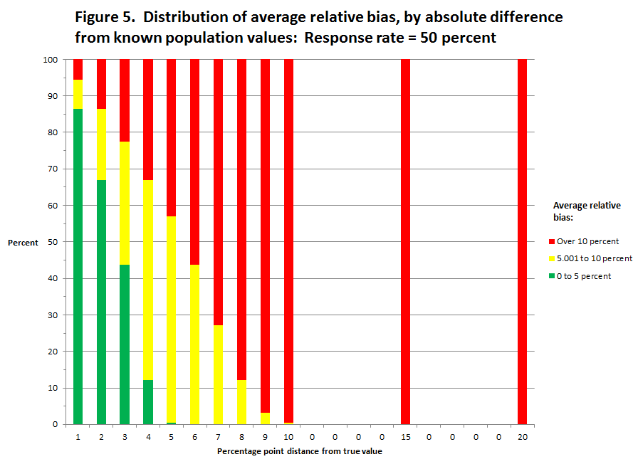
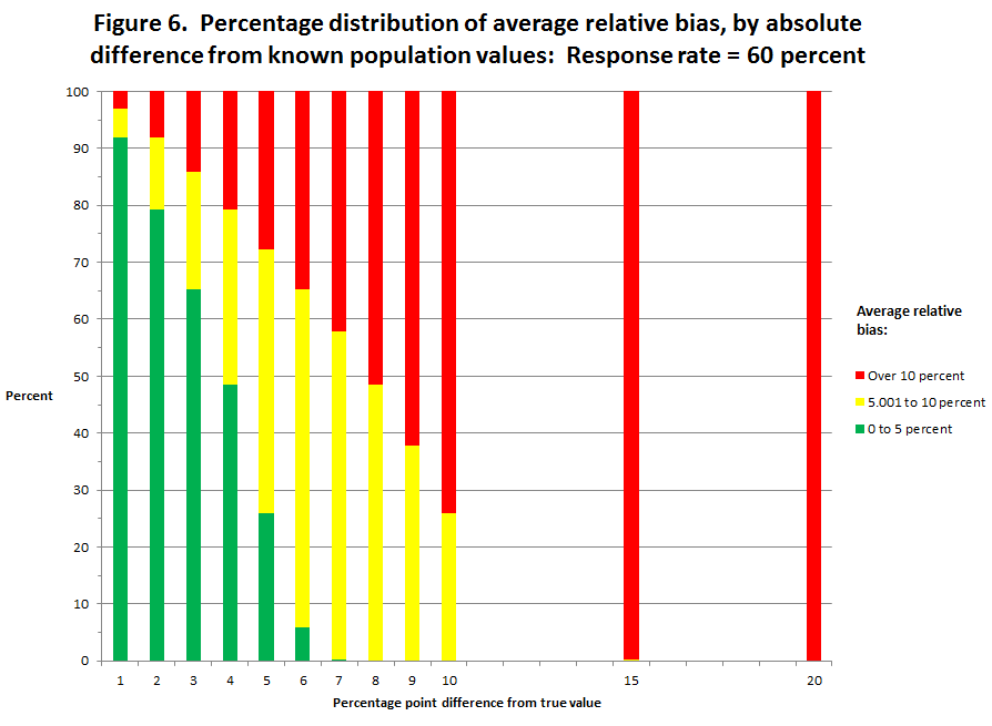
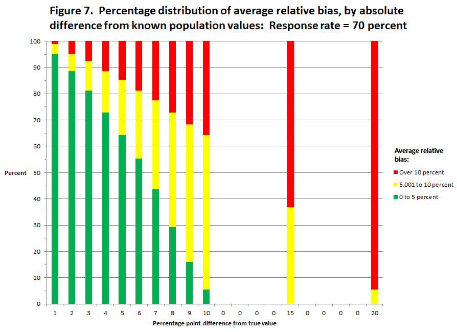
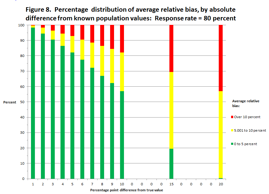
This analysis produced estimates of relative bias for each of the three variables and for the average relative bias across the three variables for each gainful employment program.8 The percentage distribution of the average relative bias estimates was plotted against the absolute value of the percentage point difference (1, 2, 3, 4, 5, 6, 7, 8, 9, 10, 15, 20) of the “what if” estimate from the true value at specific response rates (50, 60, 70, and 80 percent). These data are displayed separately for “what if” response rates of 50, 60, 70, and 80 percent (figures 5 through 8).
Looking first at figure 5, the data show that with a response rate of 50%, when the “what if” difference is set at 1 percentage point above or below the true percentage point, 86 percent of the programs have an average relative bias between 0 and 5 percent, and another 8 percent of the programs have an average relative bias between 5.001 and 10 percent; with approximately 6 percent of the programs with an average relative bias greater than 10 percent. As the size of the “what if” difference increases, the percent of programs with an average relative bias between 0 and 5 percent and between 5.001 and 10 percent both decrease while the percent of programs with an average relative bias greater than 10 percent increases. For example, with a response rate of 50 percent and a “what if” difference of 3 percentage points, 44 percent of the programs have an average relative bias between 0 and 5 percent, 34 percent of the programs have an average relative bias between 5.001 and 10 percent, and 23 percent of the programs have an average relative bias greater than 10 percent. When the “what if” difference increases to 5 percentage points, less than 1 percent of the programs have an average relative bias between 0 and 5 percent, 57 percent of the programs have an average relative bias between 5.001 and 10 percent, and 43 percent of the programs have an average relative bias greater than 10 percent. By the time the “what if” difference reaches 10 percentage points, less than 1 percent of the programs have an average relative bias less than 10 percent, and close to 100 percent of the programs have an average relative bias above 10 percent.
An examination of figures 6 through 8 shows that general relationship between the size of the “what if” difference and the percentage distribution of programs’ average relative bias holds—as the size of the “what if” difference increases, the percent of programs with an average relative bias between 0 and 5 percent and between 5.001 and 10 percent both decrease while the percent of programs with an average relative bias greater than 10 percent increases. However, at each “what if” difference, as the response rate increases the percent of the programs with an average relative bias between 0 and 10 percent increases9 and the percent of programs with an average relative bias greater than 10 percent decreases. For example, compared to a “what if” difference of 3 percentage points with a response rate of 50 percent where 78 percent of the programs have an average relative bias between 0 and 10 percent, and 23 percent of the programs have an average relative bias greater than 10 percent; with a response rate of 80 percent 97 percent of the programs have an average relative bias between 0 and 10 percent, and less than 4 percent have an average relative bias greater than 10 percent. As another example, recall that with a response rate of 50 percent and a “what if” difference of 10 points, less than 1 percent of the programs have an average relative bias of less than 10 percent; however, with a response rate of 80 percent and a “what if” difference of 10 points, 82 percent of the programs have an average relative bias of less than 10 percent. Our review of these distributions, coupled with the reported expectation that the accepted response rates are likely to be close to 50 percent, led to the addition of the criteria of relative bias value of less than 10 percent.
Table 1: Pearson r product-moment correlation coefficients for select NSLDS variables for use in potential bias analysis in Earnings and Employment Survey: 2008/2009 cohort
|
2011 Earnings |
Percentage Pell |
Percentage zero EFC |
Percentage married |
Percentage independent |
Percentage veterans |
Percentage over 24 |
Percentage female |
Percentage with mom with a BA |
Percentage with dad with a BA |
2011 Earnings |
1 |
|
|
|
|
|
|
|
|
|
Percentage Pell |
-.611 |
1 |
|
|
|
|
|
|
|
|
Percentage zero EFC |
-.593 |
.838 |
1 |
|
|
|
|
|
|
|
Percentage who are married |
.205 |
.103 |
.099 |
1 |
|
|
|
|
|
|
Percentage independent |
-.015 |
.306 |
.346 |
.764 |
1 |
|
|
|
|
|
Percentage veterans |
.440 |
-.279 |
-.316 |
.240 |
.159 |
1 |
|
|
|
|
Percentage over 24 |
.122 |
.104 |
.153 |
.774 |
.911 |
.255 |
1 |
|
|
|
Percentage female |
-.267 |
.266 |
.244 |
.208 |
.290 |
-.457 |
.106 |
1 |
|
|
Percentage with mom with a BA |
.327 |
-.545 |
-.593 |
-.307 |
-.442 |
.098 |
-.328 |
-.186 |
1 |
|
Percentage with dad with a BA |
.431 |
-.640 |
-.658 |
-.181 |
-.360 |
.148 |
-.212 |
-.183 |
.827 |
1 |
Source: National Student Loan Data System Gainful Employment Analysis Data File, Office of Program Evaluation and Policy Development |
|
|||||||||
Table 2: Beta coefficients, standard errors, and variance inflation factors for linear regression on 2011 earnings using select variables from NSLDS: 2008/2009 cohort
|
Beta |
t |
p-value |
|
Variance inflation factor |
Percentage Pell |
-.365 |
-20.359 |
0.000 |
|
3.680 |
|
(.018) |
|
|
|
|
Percentage zero EFC |
-.207 |
-10.874 |
0.000 |
|
4.131 |
|
(.019) |
|
|
|
|
Percentage who are married |
.285 |
18.031 |
0.000 |
|
2.853 |
|
(.016) |
|
|
|
|
Percentage independent |
.146 |
4.743 |
0.000 |
|
10.851 |
|
(.031) |
|
|
|
|
Percentage veterans |
.161 |
13.140 |
0.000 |
|
1.715 |
|
(.012) |
|
|
|
|
Percentage over 24 |
-.176 |
-6.218 |
0.000 |
|
9.148 |
|
(.028) |
|
|
|
|
Percentage female |
-.115 |
-9.109 |
0.000 |
|
1.812 |
|
(.013) |
|
|
|
|
Percentage with mom with a BA |
-.020 |
-1.153 |
0.249 |
|
3.532 |
|
(.018) |
|
|
|
|
Percentage with dad with a BA |
.100 |
5.438 |
0.000 |
|
3.874 |
|
(.018) |
|
|
|
|
Constant |
|
36.610 |
0.000 |
|
|
|
|
|
|
|
|
Diagnostic Statistics |
|
|
|
|
|
Number of observations |
|
|
5,524 |
|
|
F (9, 5515) |
|
|
658.95 |
*** |
|
R-squared |
|
|
0.518 |
|
|
Adjusted R-squared |
|
|
0.517 |
|
|
*** p<.001 NOTE: Standard errors are in parentheses. Source: National Student Loan Data System Gainful Employment Analysis Data File, Office of Program Evaluation and Policy Development |
|
|
|||
Table 3: Mean, median, and mode of percentage of program graduates by available NSLDS variables: 2008/2009 cohort
|
Percentage Pell |
Percentage zero EFC |
Percentage married |
Percentage independent |
Percentage veterans |
Percentage over 24 |
Percentage female |
Percentage with mom with a BA |
Percentage with dad with a BA |
Mean |
75.3 |
42.0 |
22.0 |
53.8 |
3.3 |
41.7 |
67.0 |
26.3 |
22.7 |
Median |
78.5 |
40.2 |
20.9 |
56.4 |
1.9 |
41.7 |
81.4 |
25.0 |
20.4 |
Mode |
100.0 |
50.0 |
0.0 |
66.7 |
0.0 |
50.0 |
100.0 |
33.3 |
20.0 |
|
|
|
|
|
|
|
|
|
|
Source: National Student Loan Data System Gainful Employment Analysis Data File, Office of Program Evaluation and Policy Development |
|||||||||
Table 4: Beta coefficients, standard errors, and variance inflation factors for linear regression on 2011 earnings using select variables from NSLDS without veterans:
2008/2009 cohort
|
Beta |
t |
p-value |
|
Variance inflation factor |
Percentage Pell |
-.366 |
-20.088 |
0.000 |
|
3.680 |
|
(.018) |
|
|
|
|
Percentage zero EFC |
-.264 |
-14.040 |
0.000 |
|
3.915 |
|
(.019) |
|
|
|
|
Percentage who are married |
.313 |
19.744 |
0.000 |
|
2.798 |
|
(.016) |
|
|
|
|
Percentage independent |
.231 |
7.574 |
0.000 |
|
10.367 |
|
(.031) |
|
|
|
|
Percentage over 24 |
-.217 |
-7.609 |
0.000 |
|
9.035 |
|
(.029) |
|
|
|
|
Percentage female |
-.201 |
-18.411 |
0.000 |
|
1.320 |
|
(.011) |
|
|
|
|
Percentage with mom with a BA |
-.018 |
-.993 |
0.321 |
|
3.532 |
|
(.018) |
|
|
|
|
Percentage with dad with a BA |
.095 |
5.097 |
0.000 |
|
3.872 |
|
(.019) |
|
|
|
|
Constant |
|
39.535 |
0.000 |
|
|
|
|
|
|
|
|
Diagnostic Statistics |
|
|
|
|
|
Number of observations |
|
|
5,524 |
|
|
F (9, 5515) |
|
|
698.02 |
*** |
|
R-squared |
|
|
0.503 |
|
|
Adjusted R-squared |
|
|
0.502 |
|
|
*** p<.001 NOTE: Standard errors are in parentheses. Source: National Student Loan Data System Gainful Employment Analysis Data File, Office of Program Evaluation and Policy Development |
|
|
|||
Table 5: Product measures for the linear regression on 2011 earnings using select variables from NSLDS without veterans: 2008/2009 cohort
|
r |
Beta |
Product measure |
Percent of R2 |
Percentage Pell |
-.611 |
-.366 |
0.223 |
44.4 |
|
|
|
|
|
Percentage zero EFC |
-.593 |
-.264 |
0.156 |
31.1 |
|
|
|
|
|
Percentage who are married |
.205 |
.313 |
0.064 |
12.8 |
|
|
|
|
|
Percentage independent |
-.015 |
.231 |
-0.003 |
-0.7 |
|
|
|
|
|
Percentage over 24 |
.122 |
-.217 |
-0.026 |
-5.3 |
|
|
|
|
|
Percentage female |
-.267 |
-.201 |
0.052 |
10.7 |
|
|
|
|
|
Percentage with mom with a BA |
.327 |
-.018 |
-0.005 |
-1.2 |
|
|
|
|
|
Percentage with dad with a BA |
.431 |
.095 |
0.0410 |
8.1 |
|
|
|
|
|
R-squared |
|
|
0.503 |
|
Source: National Student Loan Data System Gainful Employment Analysis Data File, Office of Program Evaluation and Policy Development |
|
|||
Table 6: Beta coefficients, standard errors, and variance inflation factors for linear regression on 2011 earnings using the reduced variable set from NSLDS: 2008/2009 cohort
|
Beta |
t |
p-value |
|
Variance inflation factor |
Percentage Pell |
-.346 |
-19.192 |
0.000 |
|
3.571 |
|
(.018) |
|
|
|
|
Percentage zero EFC |
-.245 |
-13.350 |
0.000 |
|
3.683 |
|
(.018) |
|
|
|
|
Percentage who are married |
.313 |
31.659 |
0.000 |
|
1.073 |
|
(.010) |
|
|
|
|
Percentage female |
-.167 |
-16.557 |
0.000 |
|
1.118 |
|
(.010) |
|
|
|
|
Percentage with dad with a BA |
.074 |
5.666 |
0.000 |
|
1.894 |
|
(.013) |
|
|
|
|
Constant |
|
42.304 |
0.000 |
|
|
|
|
|
|
|
|
Number of observations |
|
|
5,524 |
|
|
F (5, 5519) |
|
|
1,092.33 |
*** |
|
R-squared |
|
|
0.497 |
|
|
Adjusted R-squared |
|
|
0.497 |
|
|
*** p<.001 NOTE: Standard errors are in parentheses. Source: National Student Loan Data System Gainful Employment Analysis Data File, Office of Program Evaluation and Policy Development |
|
|
|||
Table 7: Beta coefficients, standard errors, and variance inflation factors for linear regression on 2011 earnings using the final variable set from NSLDS: 2008/2009 cohort
|
Beta |
t |
p-value |
|
Variance inflation factor |
Percentage Pell |
-.360 |
-18.805 |
0.000 |
|
3.410 |
|
(.019) |
|
|
|
|
Percentage zero EFC |
-.265 |
-13.939 |
0.000 |
|
3.369 |
|
(.019) |
|
|
|
|
Percentage female |
-.107 |
-9.918 |
0.000 |
|
1.078 |
|
(.011) |
|
|
|
|
Constant |
|
70.389 |
0.000 |
|
|
|
|
|
|
|
|
Number of observations |
|
|
5,524 |
|
|
F (3, 5521) |
|
|
1,258.11 |
*** |
|
R-squared |
|
|
0.406 |
|
|
Adjusted R-squared |
|
|
0.406 |
|
|
*** p<.001 NOTE: Standard errors are in parentheses. Source: National Student Loan Data System Gainful Employment Analysis Data File, Office of Program Evaluation and Policy Development |
|
|
|||
Graduate Employment and Earnings Survey
The purpose of the Recent Graduates Employment and Earnings Survey is to collect information about the average earnings of graduates from programs whose students receive federal financial aid and which are subject to regulations on gainful employment.
The information you provide on this survey will be grouped with information from other graduates of your program. Average earnings for all graduates of the program will be calculated and reported to the U.S. Department of Education. Your individual earnings will never be reported, disclosed, or used in any other manner.
Please verify that you are <First-Name Last-Name>. Is this correct? If you have legally changed your name but once went by <First-Name Last-Name>, please answer Yes below.
☐ No Thank you. Please return the survey in the enclosed envelope so that we can remove you from our list and you are not contacted again.
☐ Yes
The next few questions are about earnings during the <earnings year> calendar year.
This survey asks about wages and self-employment income separately. In some cases, it may not be clear to you where earnings you received should be reported. Please just use your best judgment about this, but please do NOT report the same earnings more than once. Remember to include earnings from ALL jobs.
Did you receive any wages, salary, tips, overtime pay, bonuses, or commissions from an employer in <earnings year>?
☐ No Skip to question 3.
☐ Yes2a. Think about the job you held the longest during <earnings year>.
In total, how much did you earn from that employer, before taxes and other deductions, in <earnings year>?
$_____________
2b. Now think about all OTHER jobs you held during <earnings year>.
In total, how much did you receive from all other employers, before taxes and other deductions, in <earnings year>? If you had no additional jobs, please enter a zero.
$_____________
Excluding any income mentioned above, did you receive any self-employment income, including income from your own business, in <earnings year>?
☐ No Skip to question 4.
☐ Yes 3a. What was the amount you received in net self-employment income
in <earnings year>? Please report income minus expenses. If this amount is negative, please enter zero.
$_____________
People sometimes earn extra money doing work outside of their regular jobs, such as freelancing, consulting, moonlighting, or doing other casual jobs. In <earnings year>, did you earn any other money from work you did that you have not already reported on this survey?
☐ No Thank you. Please return the survey in the envelope provided.
☐ Yes 4a. What was the amount of your additional earnings from work in
<earnings year> that are not already reported above?
$_____________ .
1 The 50 percent cut point was set for consistency with the other alternative earnings source that is allowable under the GE regulations. Specifically, the regulations require the availability of earnings data from state employment records for at least 50 percent of the students in the program’s cohort of graduates.
2 The requirement for a nonresponse bias analysis when the response rate falls below 80 percent is consistent with the OMB Standards and Guidelines for statistical surveys. While the RGEES is intended for policy rather than statistical usage, the use of the data rises to the OMB Information Quality Guidelines of influential. As such the use of this standard for statistical data collections is appropriate.
3 Programs with graduating cohorts of at less than 30 graduates over a 2- or 4-year period are not subject to the GE regulations and thus are not included in this analysis.
4 This discussion was adapted from a Memo from Chris Chapman
5 On average, in the programs included in the analysis 3.3 percent of the graduates are Veterans. A difference of 1.1 percentage point between the observed versus the actual estimate yields a relative bias of 33 percent. By way of comparison, the same size difference (i.e.,1.1 percentage point) yields a relative bias of 5 percent for the percent of graduates who were married while enrolled and a relative bias of 1.5 percent for the percent of graduates who received Pell Grants.
6 Two additional models were run including each of these two collinear variables separately. In each case 6 percent of the R2 of the overall model was accounted for.
7 Recall that 50 percent is the minimum acceptable unit response rate for RGEES, with a requirement for a nonresponse bias analysis if the unit response rate falls between 50 and 80 percent.
8 In keeping with the GE regulations programs with fewer than 30 graduates were excluded from the analysis, Thus, the second “what if” analysis was based on 5,537 GE programs with sufficient numbers of graduates and with data on the three variables used in the analysis.
9 Note also, that the percent of programs with an average relative bias between 0 and 5 percent increases disproportionate to the percent of programs with a relative bias between 5.001 and 10 percent.
| File Type | application/vnd.openxmlformats-officedocument.wordprocessingml.document |
| Author | Seastrom, Marilyn |
| File Modified | 0000-00-00 |
| File Created | 2021-01-24 |
© 2026 OMB.report | Privacy Policy